The reliance of scientific literature on p-values to test statistical significance has become quite controversial in recent years. What are p-values and how can we avoid misinterpreting them?
What is the P-Value?
The p-value has become a core statistic of frequentist hypothesis testing in all forms of science, from medical journals to econometrics. The p-value is used to describe the difference between the observed data (often from experiments) and a null hypothesis1. The null hypothesis is a straw-man hypothesis where there is no true effect or impact – e.g. the treatment being applied to patients has no significant effect on the disease of interest. In contrast, the alternative hypothesis postulates that there is a true effect by the experimental treatment – e.g. the treatment significantly improves a measure of the disease of interest.
More specifically, the p-value is the “probability of obtaining the data (or data showing as or greater difference from the null hypothesis) if the null hypothesis were true”1 (pp. 336).
In practical terms, the p-value can be used to assess the whether the observed results are consistent with the null hypothesis1. The smaller the p-value, the stronger the evidence that the observed data is inconsistent with the null hypothesis, hence if the p-value is past a certain threshold (significance level) we may reject the null hypothesis in favour of the alternative hypothesis. In biological research, the common convention is to use a 95% significance level where a result is deemed significant if the p-value is 0.05 or less.
Note that if the p-value is greater than the critical probability we say this is evidence to not reject the null hypothesis rather than accept the null hypothesis1. The p-value does not assess the probability of the null hypothesis being true because its very definition assumes the null hypothesis is true.
A Worked Example: The PlantGrowth Dataset
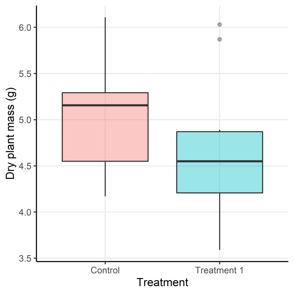
As with most statistics, the role of p-values is best demonstrated by an example of hypothesis testing. The following example draws on data simulated from an imagined experiment on plant growth (n=20), comparing the resultant plant weight (in dry mass) of a control group compared to an imagined treatment (e.g. addition of herbicide, changes to soil or light conditions)2.
Our null hypothesis (H0) is that there is no significant difference between the mean dry mass of the control plants compared to the treatment 1 plants.
In direct contrast, the alternative hypothesis (HA) is that there is a significant difference between the mean dry mass of the control and treatment 1 plants.
An initial look at the distribution of plant dry masses (Figure 1) suggests that, on average, plants in treatment 1 do have a reduced dry mass compared to those in the control group. But is this reduction in plant mass statistically significant or not? I.e. do the dry masses of plants in treatment 1 differ from the expected masses (control group) enough to reject the null hypothesis or are the differences due to chance alone?
In this comparison of mean dry mass values we can use the Welch t-test to test if there is a significant difference or not1,3. The Welch t-test is used here as the two groups (control and treatment 1) have unequal variances. This test also assumes that each plant is independent of the next and that the dry mass data is normally distributed. The output of the Welch t-test on the PlantGrowth dataset in R are printed below:
	Welch Two Sample t-test

data:  trt1 and ctrl
t = -1.1913, df = 16.524, p-value = 0.2504
alternative hypothesis: true difference in means is not equal to 0
95 percent confidence interval:
 -1.0295162  0.2875162
sample estimates:
mean of x mean of y
    4.661     5.032
The results from the t-test above are consistent with there being no significant difference between the mean plant mass of plants under treatment 1 (4.66g) compared to control group plants (5.03g) (t = -1.19, df = 16.5, p = 0.25). By definition, this p-value means that the probability that the test statistic from the t-test or less (≤-1.19) was generated under the null hypothesis is 0.251. Since this observed p-value (0.25) is larger than the conventional p-value for significance (0.05), there is evidence to not reject the null hypothesis.
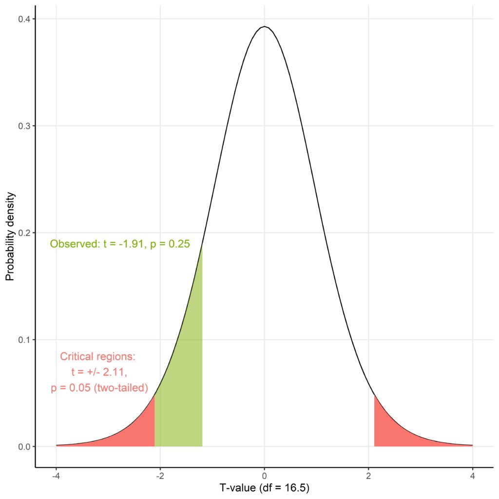
This is perhaps more easily understood graphically. Figure 2 shows the t-distribution for the 16.5 degrees of freedom (df) of this particular t-test where the areas under the curve represent the probability of that t-value being generated by the null hypothesis. The red areas are the critical regions which together cover an area equivalent to p = 0.05, meaning that the observed t-value would have to fall within these ranges to be deemed significant. Since the observed t-value does not fall within these ranges, and covers a greater region under the curve (green), it results in a larger, nonsignificant p-value.
The biological relevance of these statistics is that we have shown evidence that treatment 1 has no significant effect on plant growth compared to the control group. However, it is still worth noting that there was a nonsignificant difference in mean plant masses of -0.371g with a 95% confidence interval of -1.03g to 0.288g. A larger sample size, particularly as only 20 plants were used here2, might reveal a significant difference1,4. Then again, the nonsignificant difference was still rather small and so may not be of interest to the scientists studying plant growth.
Problems with P-Values
An article explaining p-values could not be complete without considering the common mistakes that are made in interpreting p-values and how this contributes to the loss of scientific reproducibility.
The p-value was originally invented by R.A. Fisher in the 1920s as a simple way to initially judge whether experimental results are ‘significant’ or not5. However, this use of ‘significance’ was in the old sense, i.e. to check if initial experiments are worth a second look (follow-up experiments). Fisher never really intended p-values for use in hypothesis testing. Despite this, the p-value later became associated with the rule-based statistical system of Neyman and Pearson (rivals of Fisher) for a concise method of hypothesis testing in the sciences.
The awkward history of the p-value has contributed to one of the most frequent misconceptions about the p-value: that the p-value describes the likelihood of the null hypothesis being true5,6. The p-value already assumes the null hypothesis is true, by definition, and does not incorporate any information about how realistic the null or alternative hypotheses might be. The p-value should be used to assess the statistical consistency of observed data with the null hypothesis, not whether or not the null hypothesis is true. This is one major reason that there has been a recent push for Bayesian approaches to replace p-values in scientific literature, since Bayes’ theorem can incorporate the relative likelihood that the observed data was generated by the null vs. alternative hypothesis5.
With all this focus on statistical significance it is clear how p-values can detract from the effect size seem in experimental results1,4,5,6. An effect may be significant but small, so not actually clinically or practically relevant. On the other hand, a big effect that is not found to be significant in a small study may be worth investigating in larger studies (following Fisher’s original use for the p-value). However, almost any effect can be statistically significant with a sufficiently large sample size. Reporting the effect sizes and confidence intervals should help to return our focus to the effect size.
The reliance of modern science on p-values also contributes to the so-called reproducibility crisis, a phenomenon where many published effects in scientific literature cannot be reproduced and so may not be real5. The practise of p-hacking, where researchers repeatedly try different approaches until a significant p-value is achieved, could partly account for the failure to reproduce scientific results. P-hacking is especially an issue in modern academia where many studies are searching for small effects in noisy data, such as that produced by inherently-noisy biological systems.
References
- Whitlock, MC. And Schluter, D. (2020) The Analysis of Biological Data. 3rd ed. New York, NY, USA: WH Freeman.
- Howson, I. (2021) PlantGrowth: Results from an Experiment on Plant Growth. rdrr.io. [Website] Available from: https://rdrr.io/r/datasets/PlantGrowth.html
- Spector, P. (2021) Using t-tests in R. Berkeley Statistics. [Website] Available from: https://statistics.berkeley.edu/computing/r-t-tests
- Sullivan, GM. and Feinn, R. (2012) Using Effect Size – or Why the P Value Is Not Enough. Journal of Graduate Medical Education. [Online] 4(3), 279-282. Available from: https://meridian.allenpress.com/jgme/article/4/3/279/200435/Using-Effect-Size-or-Why-the-P-Value-Is-Not-Enough
- Nuzzo, R. (2014) Scientific method: statistical errors. Nature. [Online] 506(7487), 150-152. Available from: https://pubmed.ncbi.nlm.nih.gov/24522584/
- Goodman, S. (2008) A dirty dozen: twelve p-value misconceptions. Seminars in Hematology. [Online] 45(3), 135-140. Available from: https://pubmed.ncbi.nlm.nih.gov/18582619/